by Chris Korda, Oct. 31 2012
The IPCC's Fifth Assessment Report (AR5) includes climate change scenarios called Representative Concentration Pathways (RCP), which are intended to replace the SRES scenarios given in AR4. Though AR5 won't be published until 2014, its data was finalized in 2009 and is already available [1]. Unlike the AR4 scenarios, the RCP scenarios don't provide temperature data: only forcing, emissions, and concentrations data are supplied. The omission may be partly explained by the fact that accurately deriving temperature change from forcing is a non-trivial undertaking and still an active area of research. The 2011 NASA/GISS paper Earth's energy imbalance and implications by Hansen et al. proposes a relatively straightforward method, but only applies it to historical data. Here we attempt to apply their method to RCP data, in order to answer the following specific question:
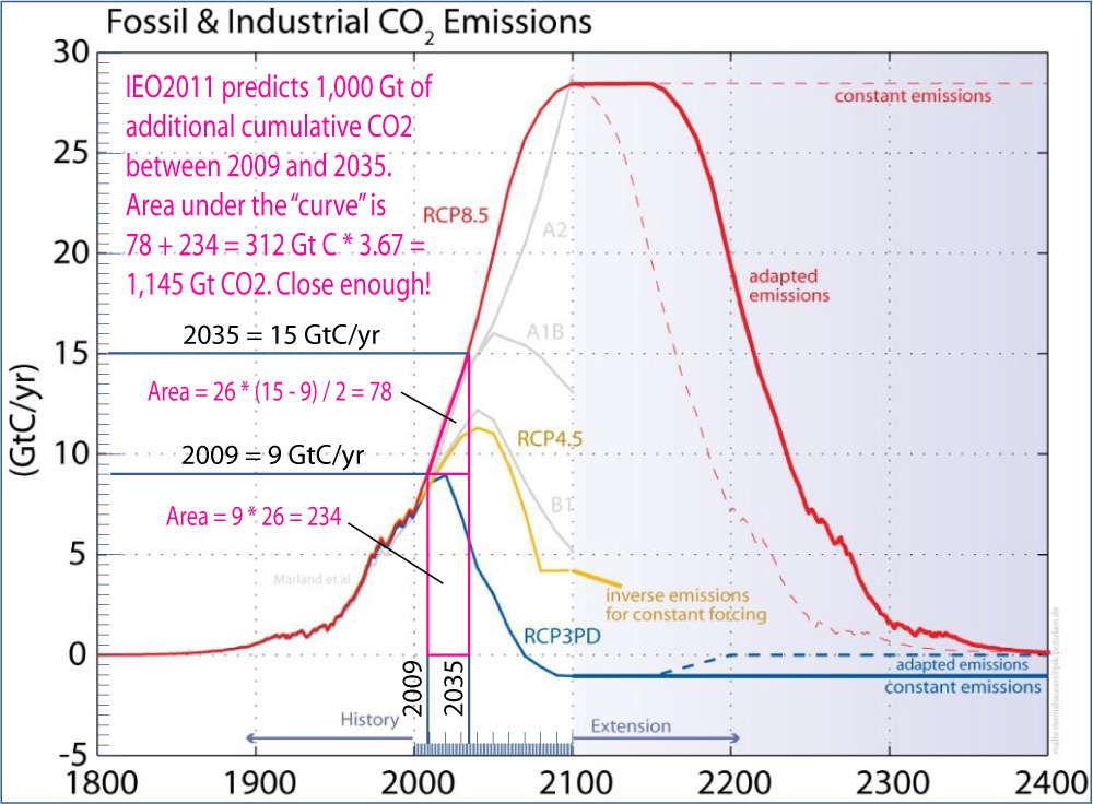
Assuming the IEO2011 Reference case of "1 trillion metric tons of additional cumulative energy-related carbon dioxide emissions between 2009 and 2035" [2], and given that this case equates to following RCP8.5 until 2035 as demonstrated by this annotated RCP8.5 chart, what increase in average global surface temperature relative to pre-industrial would result by 2035?
In the absence of inertia, the instantaneous temperature change resulting from a given year's forcing can be approximated as:
log(Concentration[iYear] / Concentration[0]) / log(2) * ClimateSensitivity
Where Concentration is an array of annual absolute CO2 concentration values in ppm, iYear is the index of the year in question, and climate sensitivity is a constant, for which 3ºC is the best estimate [3]. This instantaneous temperature change is unrealistic however, as it doesn't account for thermal inertia, particularly of the ocean, which significantly slows the response.
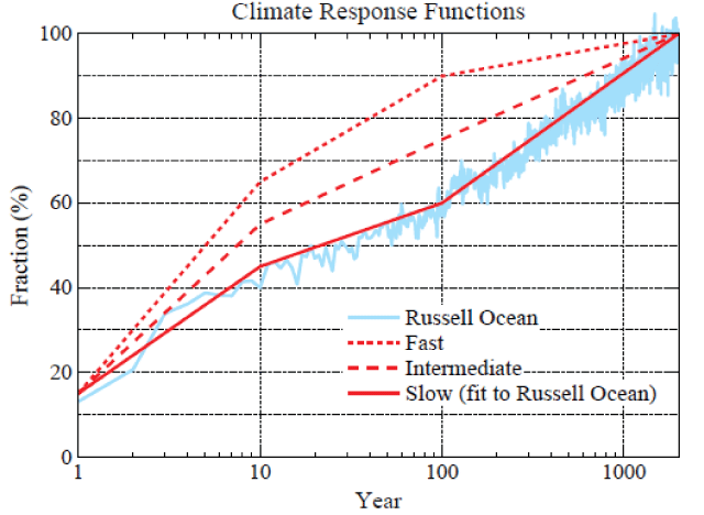
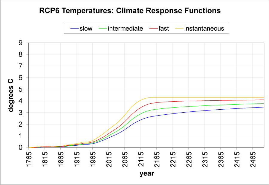
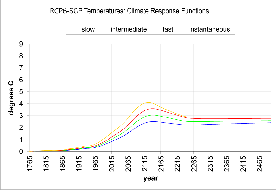
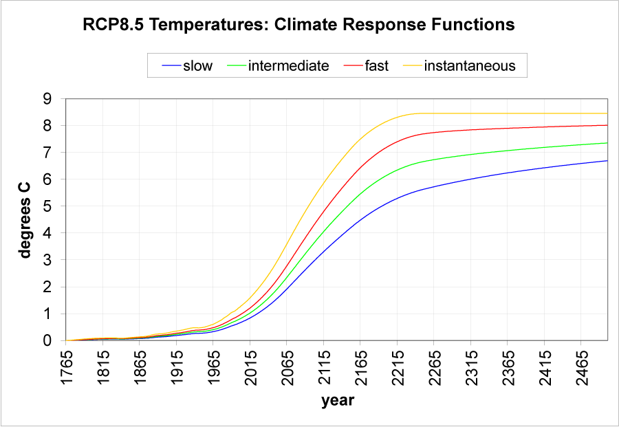
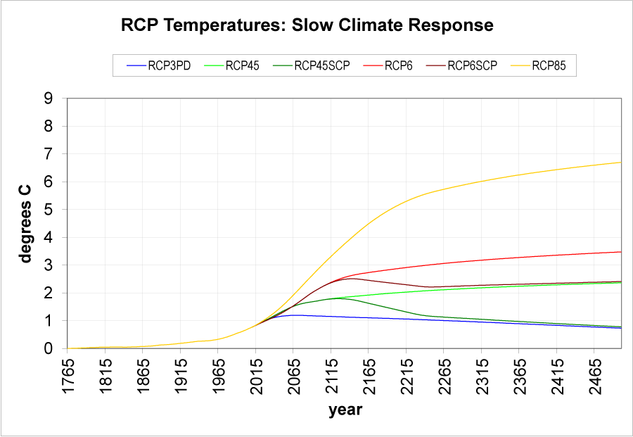
Hansen et al. model thermal inertia using a Climate Response Function, which distributes a given instantaneous temperature change forward in time, in decreasing amounts over the next two millennia. Three functions are described: slow (approximating the response of most current climate models), intermediate (the case Hansen et al. consider more likely), and fast (the upper bound). Each function is a series of decreasing percentages, defined by a three-segment polyline in log space. They're illustrated graphically in Hansen at al.'s Figure 5, and provided as interpolated annual data here.
The Climate Response Function can be applied to RCP concentration data using an iterative summing method. An array of annual temperature "buckets" is created, one for each year of the model, all initialized to zero. For each yearly CO2 concentration, the instantaneous temperature change is computed as described above. The instantaneous temperature change is then divided into 2,000 annual installments of decreasing size as determined by the Climate Response Function percentages. Each annual temperature installment is then added to the appropriate temperature bucket, spanning the following 2,000 years. This procedure is repeated for all the CO2 concentrations, moving the 2,000-year window forward by a year each time.
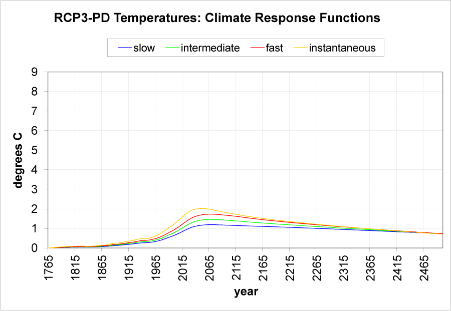
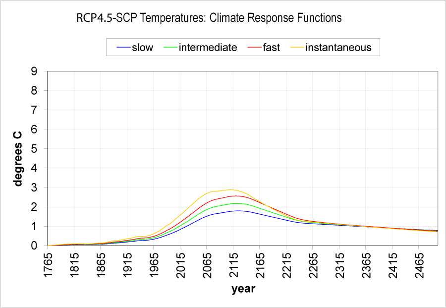
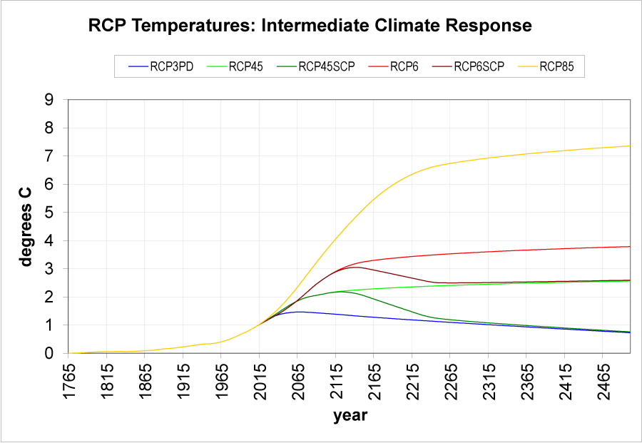
The results are divided into two groups. This first group has one plot per RCP scenario, and shows how that RCP is affected by each of Hansen at al.'s Climate Response Functions: RCP3-PD, RCP4.5, RCP4.5-SCP, RCP6, RCP6-SCP, and RCP8.5. The second group has one plot per CRF, and shows that CRF's effect on each of the RCPs: Slow, Intermediate, Fast, and Instantaneous. All of these plots are also available as a single PDF file. The C code can be viewed here, and a zip file containing the VC++ project and all input and output data is here.
Finally, to revisit the question originally posed: Assuming the IEO2011 Reference case, what increase in average global surface temperature relative to pre-industrial would result by 2035? Depending on the choice of Climate Response Function, the answers are 1.2ºC (slow), 1.5ºC (intermediate), or 1.7ºC (fast).
Thanks to Chris Dudley and Patrick at RealClimate for helping me with this project, which turned out to be a lot more than I bargained for. For detailed discussion see RealClimate's Oct. 2012 open thread. Hansen et al. plan to apply their method to temperature projections in a future paper, so we'll be able to compare to their results at some point.
References: